 Sign In
This article is about Artificial Intelligence
Writing AI program using Python tools
By NIIT Editorial
Published on 11/08/2021
10 minutes
Well-written code can be found anywhere, but it lacks methodology, which is the most important thing in learning to write a program. In this article, we will be focusing on the models and algorithms that work on real data and produce results. In addition, we will provide step-by-step guidance on how to go about approaching a particular problem. This is a beginner’s introduction to the AI world - Iris Flowers Classification Problem.
The Dataset and Algorithm used:
The Iris Flower Classification contains 150 instances of flower, where each flower involves four attributes: sepal length, sepal width, petal length, and petal width (each in cm) and three classes that belong to setosa, vermicolor, and virginica.
The aim is to develop a classifier that accurately classifies a flower as one of the three classes based on the given four features. Since it is an AI programme, keep to the most basic algorithm that can be made to perform reasonably well in a dataset, i.e. Logistic Regression.
To summarize what exactly Logistic Regression does, refer to the dataset mentioned below:

The figure shows the admission scores of students in 2 exams and if they are admitted or not admitted to the school/college based on their scores.
Here, Logistic Regression will try to find a linear decision boundary that separates the classes the best.
A scatter plot of 2D Dataset

Logistic Regression Decision Boundary
In the above figure, LR separates the two classes prominently. But in the case of more than two classes, training of ‘n’ classifiers for each ‘n’ class and having each classifier and trying to separate one class from the rest. The technique is known as ‘one-vs-all classification’. Lastly, pick out the classifier that detects its class as the strongest and allots it as the predicted class. In the given illustration from Sklearn, the decision boundary is hard to visualize:

Getting Started:
Python and a few other modules are required for writing codes, i.e., Numpy, Matplotlib, Sklearn, and Seaborn. So, first, fire up the Command Line/ Terminal and enter the given command “pip install <module-name>” to install these modules. Next, enter “python” and then “help(‘modules’)” to check what modules are installed.
Data Analysis and Visualization:
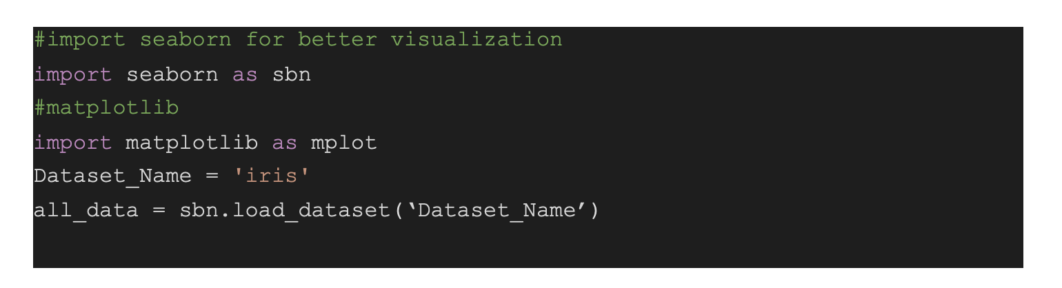
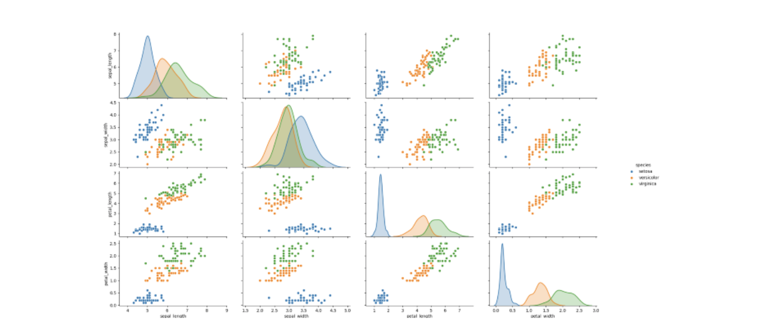
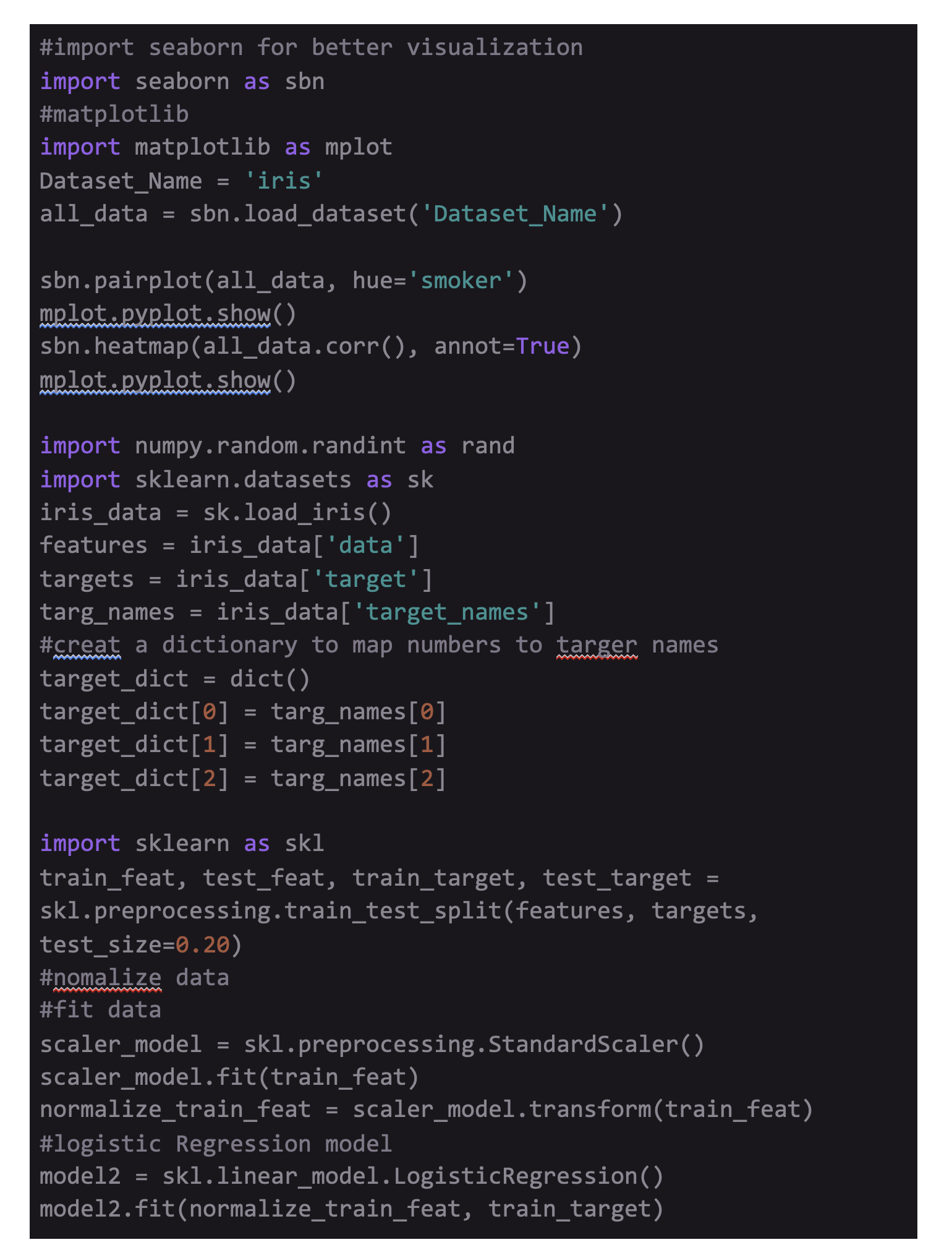
For the distribution of data in the dataset, import the matplotlib and seaborn modules and load the iris dataset included in the seaborn module.
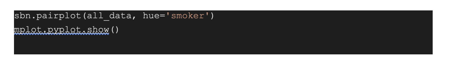
The above code will load the dataset into the dataframe ‘iris’ to visualise it much easier. Since it has four features, visualization is impossible, but some intuitions can be gained through seaborn’s powerful pairplot. Pairplot makes a scatter plot between each of the pairs of the variables in the dataset. It also distributes the value of each variable (along with the diagonal graph). Thus, it can be used to analyze which features are closely related, which are a better separator of the data, and can also be used for data distribution.
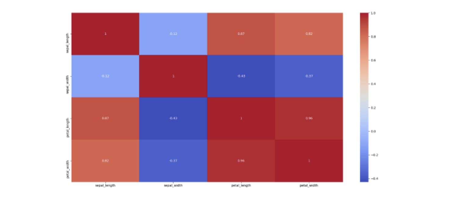
Another tool is the heatmap of correlations in Seaborn. Correlation is a statistical measure that determines the relationship between two variables' relative movements. For example, if with an increase in one variable, there is an increase in another variable and vice-versa, it is said to be positively correlated. Whereas, if with an increase in one variable, there is a decrease in other and vice-versa, then it is said to be negatively correlated. Lastly, if there is no such dependence between the variables, then they have zero correlation.
Given code shows how to plot correlations using Seaborn:

With each entry (i, j) representing the correlation between the iᵗʰ and jᵗʰ variable, iris.corr() generates 4*4 matrix. Since the dependence between i and j is the same as that of j and i, it shows that the matrix is symmetric. Also, the diagonal elements are 1, since a variable is completely dependent on itself. The annot parameter decides whether the correlation values are displayed on top of the heatmap, and colormap is set to coolwarm, which means red for high values and blue for low values.
Data Preparation and Preprocessing:
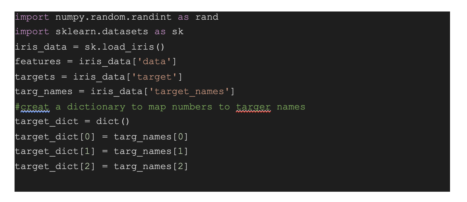
Now let’s load the data in numpy arrays and preprocess it. Preprocessing plays a vital role and enhances the performance of algorithms by a huge margin. Import the appropriate modules, and it will load the dataset in dictionary form from sklearn's iris dataset class, obtain the features and targets in numpy arrays X and Y, and the names of the classes into the name. Do the mapping from those integers to the name of the represented class. The targets in the dataset are 0, 1, and 2, which represent three classes of species. Finally, create a dictionary mapping to the flower name using the integers 0, 1, and 2.
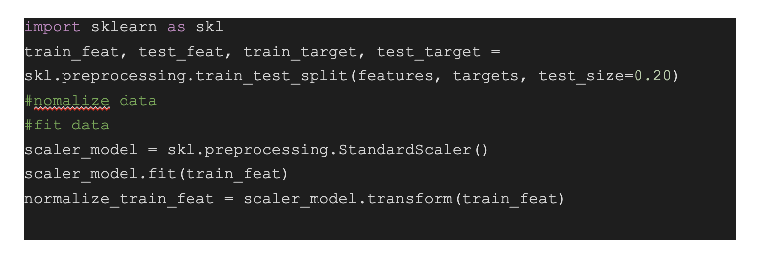
For processing, divide the data into trains using train_test_split from sklearn with the help of a test set size of 25% and use the StandardScaler class from sklearn. StandardScaler computes the mean and standard deviation for each feature in the dataset, subtracting the mean and dividing by the standard deviation. This concludes the feature of having zero mean and variance/unit standard deviation. Feature normalization helps compile all the features in the same range, and it helps optimise algorithms like gradient descent to work faster and properly.
Building the model and Evaluating it:
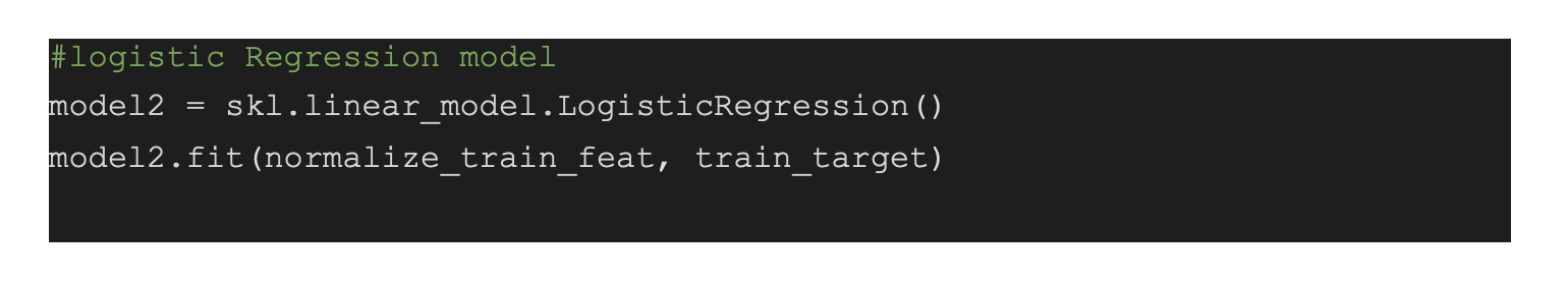
Create a code of Logistic Regression class named model, and fit in the dataset using a three line code:
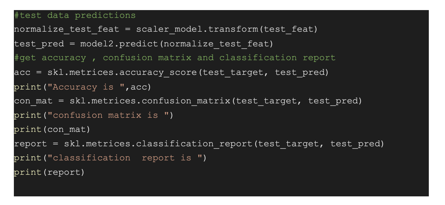
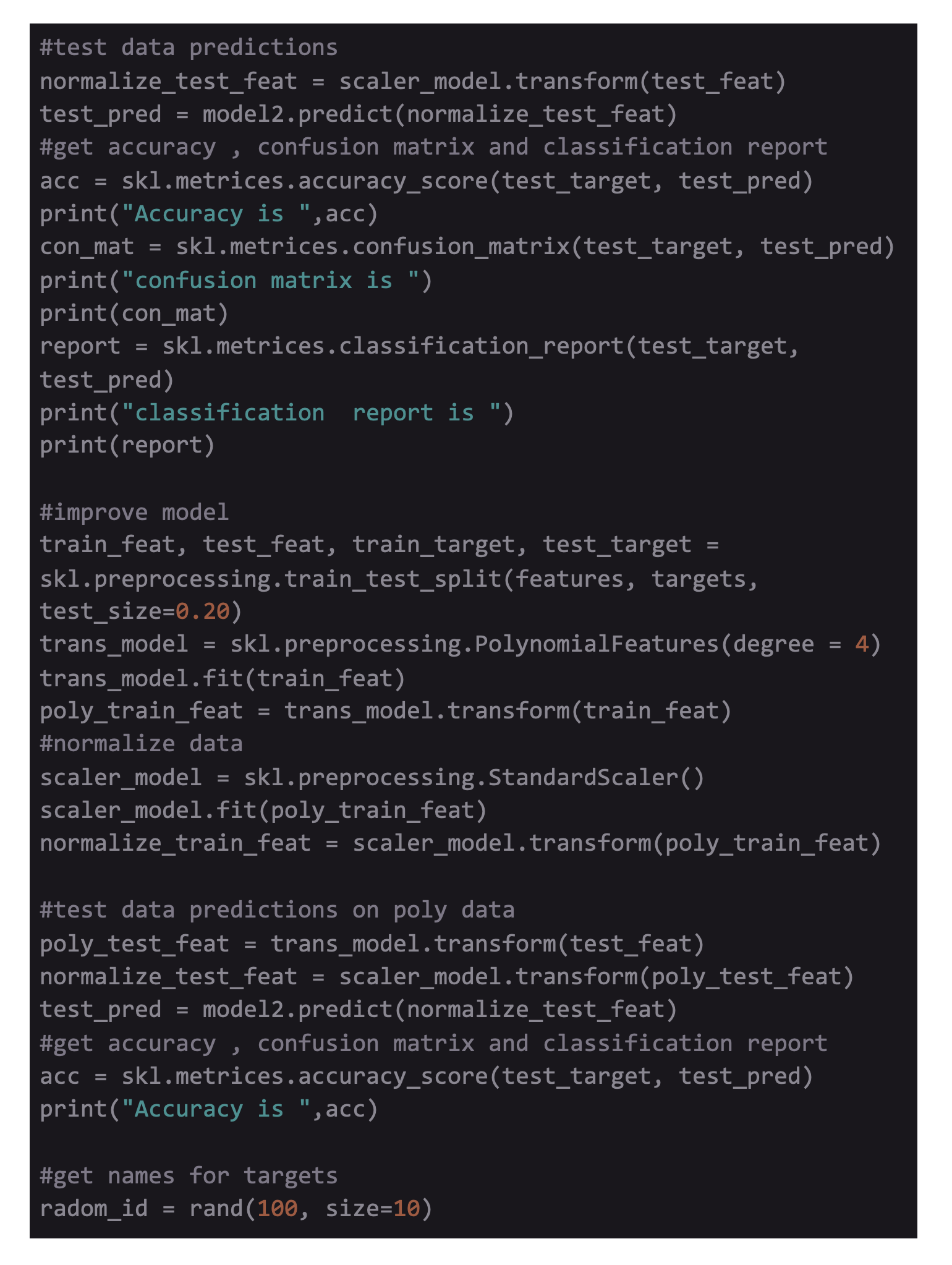
First, normalize the test set using the StandardScaler for making predictions. It is important to normalize the test set as per the mean and variance of the training set instead of the test set. To generate the 1D array of predictions, use the predict function for both training and test set. Since there are many metrics available in the metrics class of sklearn, the article will focus on the three most relevant metrics- accuracy, classification report, and confusion matrix.
Since the dataset is small, different results can be seen each time while training a model.
Output:

Here, test set accuracy is approx 94.7%, and training set accuracy is about 95.5%. Thus, for the F-1 score of all different classes in the test set, the weighted average is 0.95.
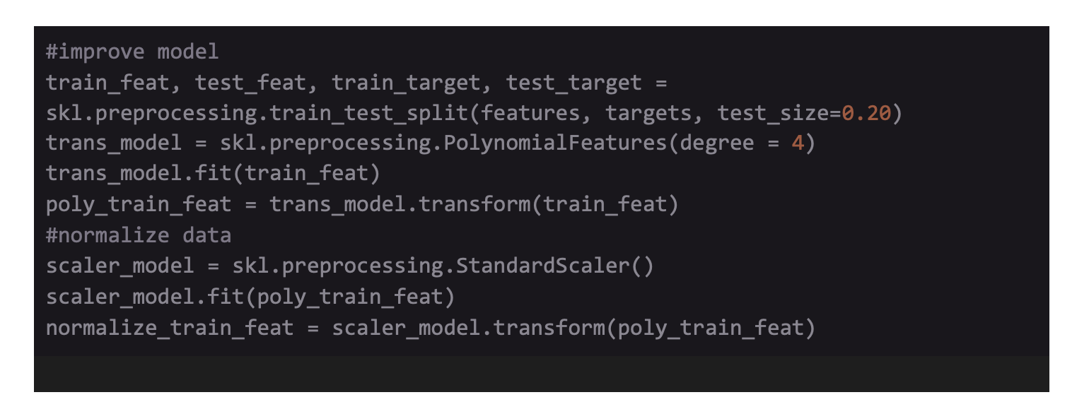
Improving the Model:
Instead of introducing a normal model, a better model can be introduced with polynomial features into the model like x₁², x₁x₂, x₂² for making a non-linear decision boundary for separating the classes. Given is the dataset:

The dataset shows the scores obtained from tests on different microchips, including the classes it belongs to. As seen from the graph, there is no linear decision boundary that can separate the data. A decision boundary is generated by using the polynomial logistic regression as shown below:
A scatter plot of 2D Dataset

Polynomial Logistic Regression Decision Boundary
Here, lambda refers to the regularization parameter. Regularization is important while dealing with non-linear models as they don’t want to overfit training sets.
PolynomialFeatures from sklearn are added in the dataset to add polynomial features. This feature will enter the preprocessing as an added step, similar to that of the normalizing step. Adjust the degree accordingly and see the effect (here 5th power degree is added). The model starts overfitting for higher degree terms and it is not needed.

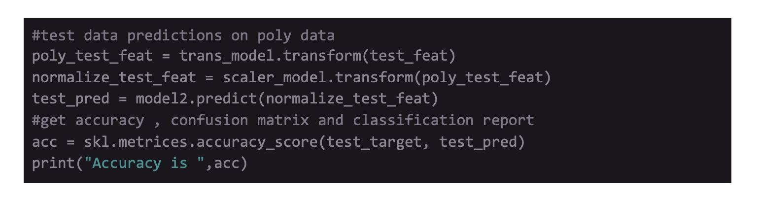
Keep continuing the above steps to fit the model. For making predictions, transform the test set using poly first.

Lastly, evaluate the model with the help of metrics discussed above. Again, the results can differ with each time the model is trained.
Output:
Here, the training set accuracy is about 92.2%, and test set accuracy is approx 97.4%. The weighted F-1 score is 0.97 on test sets which are improved, and it classifies only one incorrect example from the test set.
Generating Predictions:
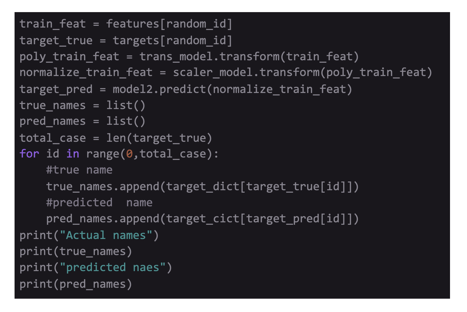
An arrangement of 4 numbers representing the four features of a flower is used that tells which species it thinks it belongs to. Then, randomly 20 examples are picked from the dataset, preprocessing is done, and classes are predicted.
Y_true represents the true class while the Y_pred is the predicted class of the example. These both are integers as the model works with numeric data. Then, create 2 lists i.e., true names and the predicted names of the species using the dictionary mapping already created of each example.
Output:
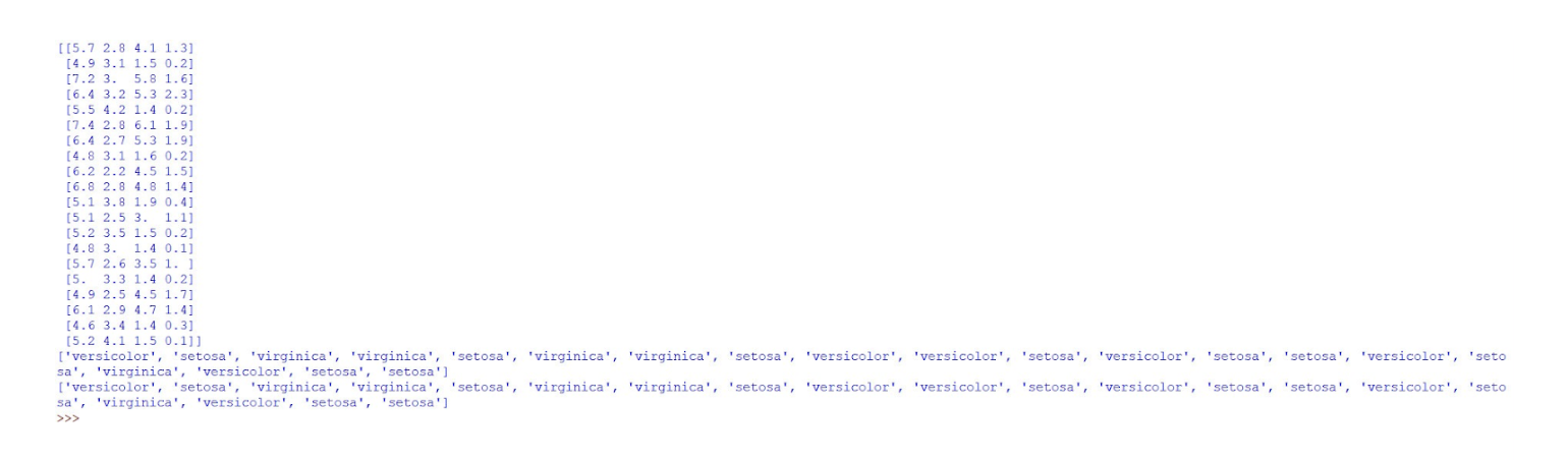
All the predictions generated are correct because of the higher accuracy in the model. Complete code of the final mode is as follows:
Conclusion:
The above article gives an idea of building a simple AI or Machine Learning model to solve a particular problem. The article includes five stages:
- Obtaining a dataset for a task.
- Analyzing and Visualizing the Dataset.
- Converting the data into a form that can be used and preprocessing it.
- Building the model and evaluating it.
- Checking where the model is getting short and improving it.
While building an Artificial Intelligence Application, a lot of trial and error is involved. If the model doesn't work, don’t be disheartened. The right dataset is crucial and is a game-changer when it comes to real-world models. To learn more about Artificial Intelligence you can opt the courses Advanced PGP in Data Science and Machine Learning (Full Time) or Advanced PGP in Data Science and Machine Learning (Part Time).
SHARE


Advanced PGP in Data Science and Machine Learning (Full Time)
Become an industry-ready StackRoute Certified Data Science professional through immersive learning of Data Analysis and Visualization, ML models, Forecasting & Predicting Models, NLP, Deep Learning and more with this Job-Assured Program with a minimum CTC of ₹5LPA*.
Job Assured Program*
Practitioner Designed