
 Sign Up
This article is about Data Science
How to start machine learning in python
By NIIT Editorial
Published on 26/08/2021
8 minutes
Machine learning involves artificial intelligence that enables the computer to learn from the given set of data and further predict the results of new data. It mainly focuses on training the computer using computer programmes that can change the result when exposed to new sets of data without being explicitly programmed. The best way to start machine learning is by investing your time in learning the basics.
Learning basic python skills
A basic understanding of python is crucial if we want to use python as a tool to perform machine learning. Python is a programming language that runs on an interpreter system. It is well known for its applicability in both research and development fields, anywhere that uses coding, mathematical computations or data. It connects to the database system which means it can read and modify files. Although it uses a simple syntax similar to the English language, it is also used for implementing and executing complex machine learning algorithms.
The first step is to install python and launch the python interpreter.
Starting with small end to end projects
The best accessible way to learn python for machine learning is to design and complete small projects. They will help build your confidence and guide you through. Learning through books and courses can be intimidating as they are filled with a lot of information but do not demonstrate how to properly implement them.
The best way to familiarise yourself with the machine learning algorithms is to work on end to end small projects. Applying it to your datasets, like loading and summarizing data, evaluating algorithms and making small predictions to gain experience on this platform. You can choose a course such as Advanced PGP in Data Science and Machine Learning (Full Time) or Advanced PGP in Data Science and Machine Learning (Part-Time) that render practical knowledge.
Once you get familiar with the template to use a series of datasets, you can work on improving result tasks.
A machine learning project has various steps namely:
- Defining the problem
- Data preparation
- Evaluation
- Improving results
- Predict
Hello world of machine learning
For beginners, The Iris dataset is the most popular machine learning project. The Iris dataset is a classification problem of iris flowers.
- It is a relatively small, simple and easier type of supervised learning algorithm, which makes it perfect for beginners.
- The attributes included are numeric allowing you to learn how to load and handle data.
- The numeric attributes are all in the same scale and same units, so it does not require complex transforms.
- It is a multi-nominal problem that may include some specialized handling.
Getting started with hello world machine learning in Python
Working through a machine learning project involves many steps :
- Install the Python and SciPy platform
- Load the dataset
- Summarizing
- Visualize the data
- Evaluating the algorithms
- Predict
Let's work through each step and understand how they work in this step by step tutorial.
1. Download, install, and start Python SciPy
Install Python and SciPy platform on your system. You need to install SciPy libraries, the libraries required for this project that you need to install are:
- SciPy
- Numpy
- Matplotlib
- Pandas
- Sklearn
There are numerous ways to install these libraries on your system, pick one method to be consistent and avoid further confusion. Keep in mind that the method of installation also varies depending on your device's operating system.
Open a command line and start the interpreter to test out your Python environment:
After installing, start the python to make sure it was installed successfully and is working properly. The following script will help to test out the installed version. It helps in importing each library required here and prints the version.
Open command line and start the python interpreter, then type or coy the following code:
# Check the versions of libraries
import sys
import scipy
import numpy
import matplotlib
import pandas
import sklearn
print('Python version')
print(format(sys.version))
print('scipy version\n')
print(format(scipy.__version__))
print('numpy version\n')
print(format(numpy.__version__))
print('matplotlib version\n')
print(format(matplotlib.__version__))
print('pandas version\n')
print(format(pandas.__version__))
print('scikit-learn\n')
print(format(sklearn.__version__))
Make sure you copy the above code clearly and precisely to get the correct output.
Python version
3.9.0 (tags/v3.9.0:9cf6752, Oct 5 2020, 15:34:40) [MSC v.1927 64 bit (AMD64)]
scipy version
1.7.0
numpy version
1.21.1
matplotlib version
3.4.2
pandas version
1.3.0
scikit-learn
0.24.2
2. Load the data
The iris dataset we are using contains 150 observations of iris flowers. The four columns showcase measurement of flowers in centimetres and the last fifth column is the classification of the flower.
Import libraries
After setting the environment as mentioned above, you need to import libraries including all the modules and functions that are required in this tutorial.
Type or copy the given script:
# Load libraries
from pandas import read_csv
from pandas.plotting import scatter_matrix as sc
import matplotlib.pyplot as plt
from sklearn.model_selection import train_test_split
from sklearn.model_selection import cross_val_score
from sklearn.model_selection import StratifiedKFold
from sklearn.metrics import classification_report
from sklearn.metrics import confusion_matrix
from sklearn.metrics import accuracy_score
from sklearn.linear_model import LogisticRegression
from sklearn.tree import DecisionTreeClassifier
from sklearn.neighbors import KNeighborsClassifier
from sklearn.discriminant_analysis import LinearDiscriminantAnalysis
from sklearn.naive_bayes import GaussianNB
from sklearn.svm import SVC
Load dataset
To load the data Pandas library is used. In this step, we are specifying the column names that will later help in exploring the data.
...
# Load dataset
column_names = ['seplen', 'sepwid', 'petlen', 'petwid', 'class']
dataset = read_csv('samplecsv.csv', names=column_names)
print(dataset)
3. Summarize
While summarizing the data, analyze the data in different ways as mentioned below:
Dimensions of the dataset
The given script will help you to understand how many instances and attributes the data contains.
...
# shape
shape=dataset.shape
print(shape)
The output should be as given below
(150, 5)
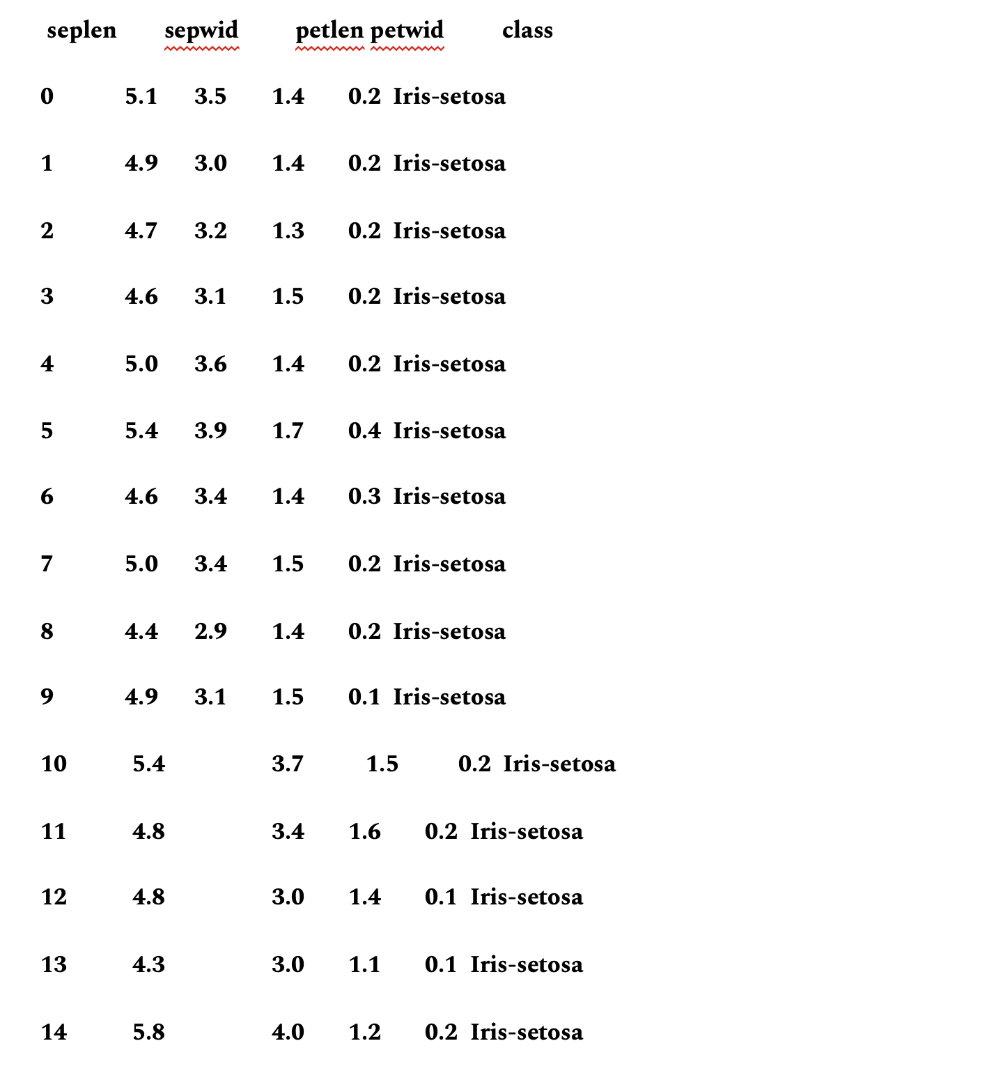
Read the data
Read and analyze the data
...
# head
head=dataset.head(15)
print(head)
The output should show the 15 rows of the data
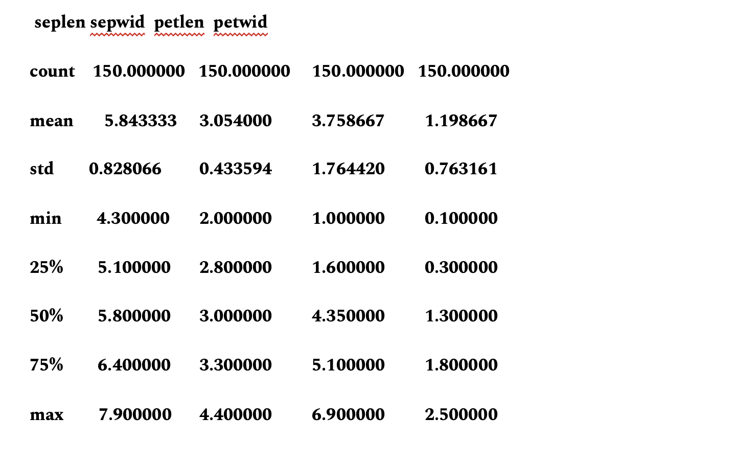
Statistical Summary of each attribute
This summary contains descriptions such as count, percentiles, mean value, maximum and minimum values.
...
# descriptions
description=dataset.describe()
print(description)
The output should be similar as below.
Class distribution
This step determines the number of instances that belong to each species. The output clearly states that each species has the same number of occurrences.
...
# class distribution
class_destribution=dataset.groupby('class').size()
print(class_destribution)
Output:
class
Iris-setosa 50
Iris-versicolor 50
Iris-virginica 50
Summarized Example
All the above-mentioned data can be summarised into one script.
# summarize the data
from pandas import read_csv
# Load dataset
column_names = ['seplen', 'sepwid’, 'petlen', 'petwid', 'class']
dataset = read_csv('samplecsv.csv', names=column_names)
# shape
shape=dataset.shape
print(shape)
# head
head=dataset.head(15)
print(head)
# descriptions
description=dataset.describe()
print(description)
# class distribution
class_destribution=dataset.groupby('class').size()
print(class_destribution)
4. Data visualization
After summarizing, data visualization is important for better analysis. It helps you understand the crucial information in the dataset.
Univariate plots are used to understand attributes and multivariate plots are used to understand structured relationships between various variables.
Univariate plots
# box plot
dataset.plot(kind='box', subplots=True, layout=(2,2))
plt.show()
This provides plots of each attribute
Histograms can also be created of each variable
..
# histograms
dataset.hist()
plt.show()
Multivariate plots
This helps to understand the relationship between various variables.
...
# scatter plot matrix
sc(dataset)
plt.show()
Complete example
The methods of data visualization can be summarised into one script for reference.
# visualize the data
from pandas import read_csv
import matplotlib.pyplot as plt
from pandas.plotting import scatter_matrix as sc
# Load dataset
column_names = ['seplen', 'sepwid', 'petlen’, 'petwid', 'class']
dataset = read_csv('samplecsv.csv', names=column_names)
# box
dataset.plot(kind='box', subplots=True, layout=(2,2))
plt.show()
# histograms
dataset.hist()
plt.show()
sc(dataset)
plt.show()
5. Evaluation of Algorithms
This step is important to evaluate the accuracy of the data.
Split Out validation dataset
The loaded dataset will be split into two. 80% of the dataset will be used to train and evaluate; the rest will be used as a validation set.
...
# Split-out validation dataset
y=dataset['class']
x=dataset.drop('class', axis=1)
x_train, x_test, y_train, y_test = train_test_split(x, y, test_size=0.20, random_state=1)
Build and evaluate models
...
# Spot Check Algorithms
x_train, x_test, y_train, y_test = train_test_split(X, Y, test_size=0.20, random_state=1)
scaler_type=StandardScaler()
scale=scaler_type.fit(x_train)
x_train=scale.transform(x_train)
x_test=scale.transform(x_test)
ml_model1=LogisticRegression()
kfold = StratifiedKFold(n_splits=10, random_state=1, shuffle=True)
cv_results = cross_val_score(ml_model1, x_train, y_train, cv=kfold, scoring='accuracy')
results.append(cv_results)
print('lr: %f (%f)' % ( cv_results.mean(), cv_results.std()))
ml_model2=LinearDiscriminantAnalysis()
kfold = StratifiedKFold(n_splits=10, random_state=1, shuffle=True)
cv_results = cross_val_score(ml_model1, x_train, y_train, cv=kfold, scoring='accuracy')
results.append(cv_results)
print('ldr %f (%f)' % ( cv_results.mean(), cv_results.std()))
ml_model3=KNeighborsClassifier()
kfold = StratifiedKFold(n_splits=10, random_state=1, shuffle=True)
cv_results = cross_val_score(ml_model3, x_train, y_train, cv=kfold, scoring='accuracy')
results.append(cv_results)
print('knn %f (%f)' % ( cv_results.mean(), cv_results.std()))
ml_model4=DecisionTreeClassifier()
kfold = StratifiedKFold(n_splits=10, random_state=1, shuffle=True)
cv_results = cross_val_score(ml_model4, x_train, y_train, cv=kfold, scoring='accuracy')
results.append(cv_results)
print('dtc %f (%f)' % ( cv_results.mean(), cv_results.std()))
ml_model5=GaussianNB()
kfold = StratifiedKFold(n_splits=10, random_state=1, shuffle=True)
cv_results = cross_val_score(ml_model5, x_train, y_train, cv=kfold, scoring='accuracy')
results.append(cv_results)
print('gnb %f (%f)' % ( cv_results.mean(), cv_results.std()))
ml_model6=SVC(gamma='auto')
kfold = StratifiedKFold(n_splits=10, random_state=1, shuffle=True)
cv_results = cross_val_score(ml_model6, x_train, y_train, cv=kfold, scoring='accuracy')
results.append(cv_results)
print('svc %f (%f)' % ( cv_results.mean(), cv_results.std()))
Output:
lr: 0.966667 (0.040825)
ldr 0.966667 (0.040825)
knn 0.950000 (0.055277)
dtc 0.933333 (0.050000)
gnb 0.950000 (0.055277)
svc 0.958333 (0.041667)
After building models, select the best model with the most accurate estimation.
You can also compare the models using the following algorithm.
...
# Compare Algorithms
names=("lr","ldr","knn","dtc","gnb","svc")
plt.boxplot(results, labels=names)
plt.title('Comparison of algo')
plt.show()
Complete example
All the above criteria can be compiled into one for reference.
from matplotlib import pyplot
from pandas import read_csv
from sklearn.model_selection import train_test_split
from sklearn.model_selection import cross_val_score
from sklearn.preprocessing import StandardScaler
import matplotlib.pyplot as plt
from sklearn.model_selection import StratifiedKFold
from sklearn.metrics import classification_report
from sklearn.metrics import confusion_matrix
from sklearn.metrics import accuracy_score
from sklearn.linear_model import LogisticRegression
from sklearn.semi_supervised.tests.test_self_training import X_train
from sklearn.semi_supervised.tests.test_self_training import y_train
from sklearn.tree import DecisionTreeClassifier
from sklearn.neighbors import KNeighborsClassifier
from sklearn.discriminant_analysis import LinearDiscriminantAnalysis
from sklearn.naive_bayes import GaussianNB
from sklearn.svm import SVC
column_names = ['seplen', 'sepwid', 'petlen', 'petwid', 'class']
dataset = read_csv('samplecsv.csv', names=column_names)
Y = dataset['class']
X = dataset.drop('class', axis=1)
results=[]
x_train, x_test, y_train, y_test = train_test_split(X, Y, test_size=0.20, random_state=1)
scaler_type=StandardScaler()
scale=scaler_type.fit(x_train)
x_train=scale.transform(x_train)
x_test=scale.transform(x_test)
ml_model1=LogisticRegression()
kfold = StratifiedKFold(n_splits=10, random_state=1, shuffle=True)
cv_results = cross_val_score(ml_model1, x_train, y_train, cv=kfold, scoring='accuracy')
results.append(cv_results)
print('lr: %f (%f)' % ( cv_results.mean(), cv_results.std()))
ml_model2=LinearDiscriminantAnalysis()
kfold = StratifiedKFold(n_splits=10, random_state=1, shuffle=True)
cv_results = cross_val_score(ml_model1, x_train, y_train, cv=kfold, scoring='accuracy')
results.append(cv_results)
print('ldr %f (%f)' % ( cv_results.mean(), cv_results.std()))
ml_model3=KNeighborsClassifier()
kfold = StratifiedKFold(n_splits=10, random_state=1, shuffle=True)
cv_results = cross_val_score(ml_model3, x_train, y_train, cv=kfold, scoring='accuracy')
results.append(cv_results)
print('knn %f (%f)' % ( cv_results.mean(), cv_results.std()))
ml_model4=DecisionTreeClassifier()
kfold = StratifiedKFold(n_splits=10, random_state=1, shuffle=True)
cv_results = cross_val_score(ml_model4, x_train, y_train, cv=kfold, scoring='accuracy')
results.append(cv_results)
print('dtc %f (%f)' % ( cv_results.mean(), cv_results.std()))
ml_model5=GaussianNB()
kfold = StratifiedKFold(n_splits=10, random_state=1, shuffle=True)
cv_results = cross_val_score(ml_model5, x_train, y_train, cv=kfold, scoring='accuracy')
results.append(cv_results)
print('gnb %f (%f)' % ( cv_results.mean(), cv_results.std()))
ml_model6=SVC(gamma='auto')
kfold = StratifiedKFold(n_splits=10, random_state=1, shuffle=True)
cv_results = cross_val_score(ml_model6, x_train, y_train, cv=kfold, scoring='accuracy')
results.append(cv_results)
print('svc %f (%f)' % ( cv_results.mean(), cv_results.std()))
names=("lr","ldr","knn","dtc","gnb","svc")
plt.boxplot(results, labels=names)
plt.title('Comparison of algo')
plt.show()
6. Predict
We will use the most accurate model to make predictions.
Make predictions on the validation set
The model chosen can be used on the entire dataset
..
# Make predictions on validation dataset
model = LogisticRegression()
model.fit(x_train, y_train)
predictions = model.predict(x_test)
print(predictions)
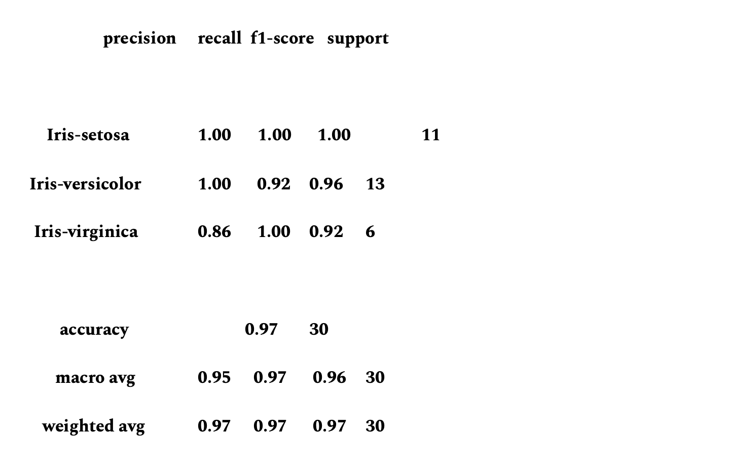
Evaluate predictions
This step is important to calculate classification accuracy and provides a confusion matrix of the errors.
....
# Evaluate predictions
accuracyscore=accuracy_score(y_test, predictions)
conf_mat=confusion_matrix(y_test, predictions)
class_report=classification_report(y_test, predictions)
print(accuracyscore)
print(conf_mat)
print(class_report)
Output:
0.9666666666666667
[[11 0 0]
[ 0 12 1]
[ 0 0 6]]
Complete example
The above-given scripts can be summarised together for reference.
# make predictions
from pandas import read_csv
from sklearn.model_selection import train_test_split
from sklearn.preprocessing import StandardScaler
from sklearn.metrics import classification_report
from sklearn.metrics import confusion_matrix
from sklearn.metrics import accuracy_score
from sklearn.linear_model import LogisticRegression
column_names = ['seplen', 'sepwid', 'petlen', 'petwid', 'class']
dataset = read_csv('samplecsv.csv', names=column_names)
Y = dataset['class']
X = dataset.drop('class', axis=1)
results=[]
x_train, x_test, y_train, y_test = train_test_split(X, Y, test_size=0.20, random_state=1)
scaler_type=StandardScaler()
scale=scaler_type.fit(x_train)
x_train=scale.transform(x_train)
x_test=scale.transform(x_test)
model = LogisticRegression()
model.fit(x_train, y_train)
predictions = model.predict(x_test)
accuracyscore=accuracy_score(y_test, predictions)
conf_mat=confusion_matrix(y_test, predictions)
class_report=classification_report(y_test, predictions)
print(accuracyscore)
print(conf_mat)
print(class_report)
Conclusion
This article will help you to create a Machine learning project with Python even if you are a beginner and have no knowledge of the platform. The best way to start with a new platform in machine learning is to complete small projects.
SHARE


Data Science Foundation Program (Full Time)
Become an industry ready StackRoute Certified Python Programmer in Data Science. The program is tailor-made for data enthusiasts. It enables learner to become job-ready to join data science practice team and gain experience to grow up as Data Analyst.
Visualise Data using Python and Excel
6 Weeks Full Time Immersive